How to conditional format entire row/column mac numbers

Conditional highlighting of Mac Numbers can only format a cell. But I receive a requirement from my boss to change the color of the entire row. So how did I do it? I will write the instructions below.

The instructions seem complicated and have a lot of steps. But they are actually simple. I can summarize the instructions into 3 tasks. The first task is to make a copy of the original table. The cells of this second table will change to blank if the requirement doesn’t meet. And creating a formula to do so is the second task. Finally, your last task is to create a conditional highlighting rule to change the format of the cell if the corresponding cells of the two tables match. Then apply the rule to all the cells of your original table. 

The detailed instructions are below.

1. How to conditional format entire row in Mac Numbers

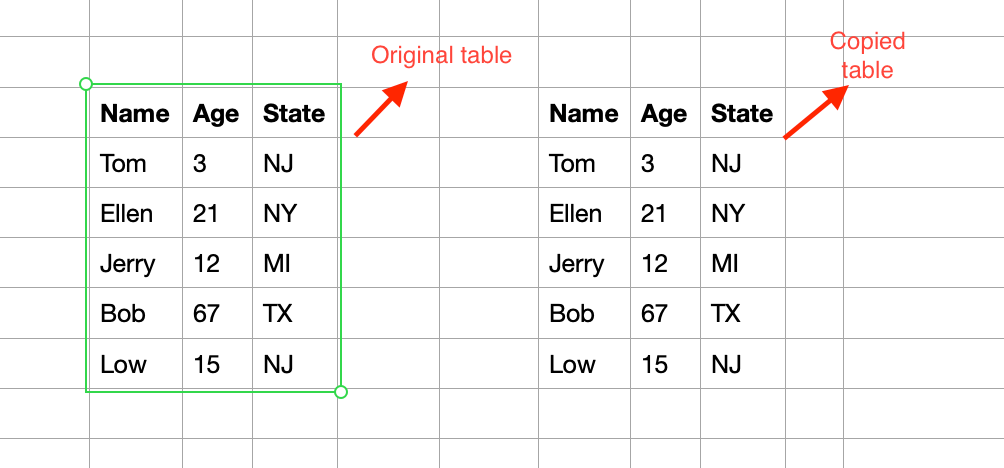
You will need a second table to achieve this task. The second table has the same size as the original table. The only difference is that the second table either has the same value as the original table or has the blank value. Simply copy and paste the original table to an empty cell in your sheet. Take a look at my example.

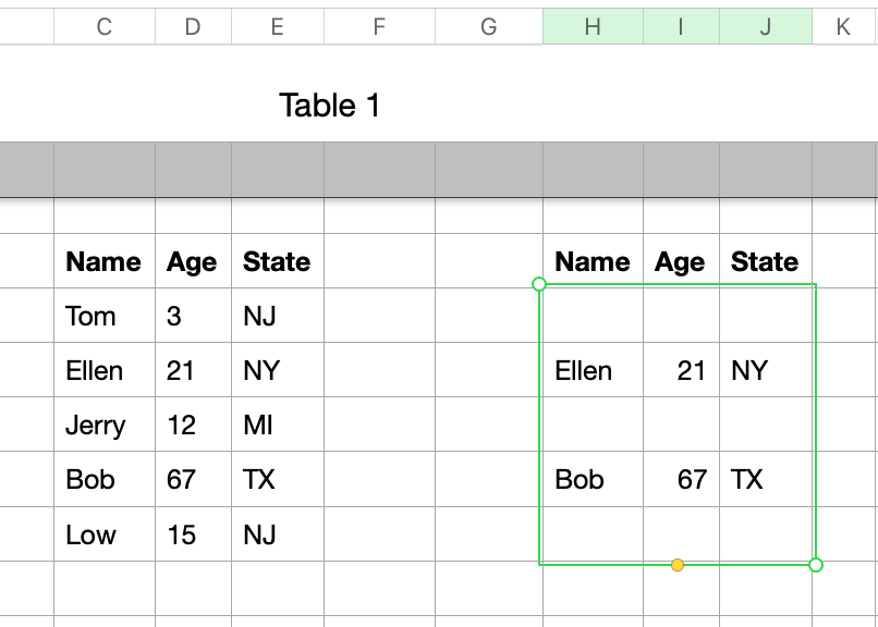
In the following task, you must turn the values of the second table to blank if your criteria doesn’t meet. I will show you how to do it in my example. Adjust the formula to match your criteria. If the person isn’t older than 21, I want to see blank values on that row of the second table. In order to do so, I use the following formula. 

D6 is the age of the person. I want the age to be greater than or equal to 21. If it is true, then take the value from the corresponding cell in the original table. Otherwise, put a blank value into the cell. Eventually, I want to copy the formula to every cell in the second table. But I don’t want Mac Numbers to change my age column. That’s why I preserve the column of the age cell. The result is below.

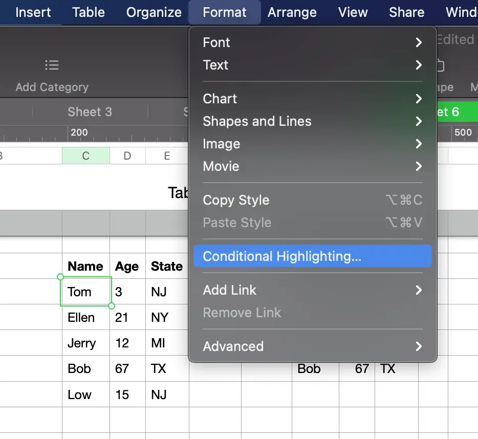
The next task is to create a conditional highlighting rule to change the format of the entire row in the original table. To do so, I select a cell in the original table, click the Format menu, and click Conditional Highlighting…

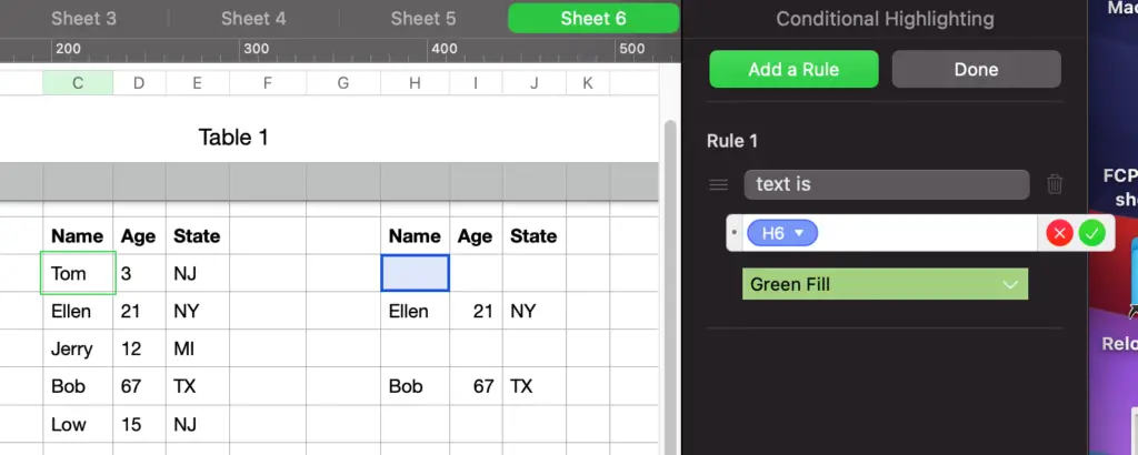
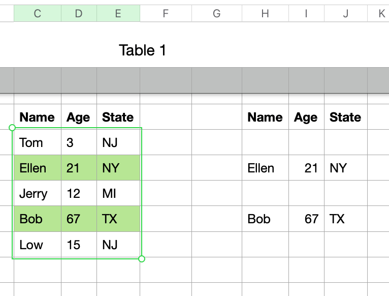
The rule is if the Text is the same as the corresponding cell in the second table, then change the format of the cell to your liking. I changed mine to green. 

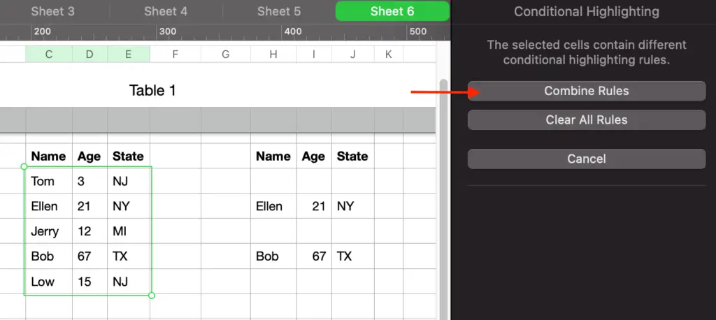
Then I select the entire original table and click the “Combine Rules” button. And complete.

The end result looks like the screenshot below. If you don’t want to see the second table, you can hide those columns. 

2. How to conditional format entire column in Mac Numbers

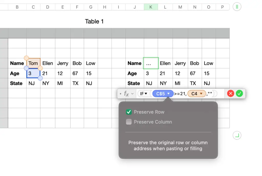
Okay, so the instruction above is to format the entire row. What about the entire column? You use a very similar approach. You only need to change one thing. That is to perverse the row instead of the column in the formula. Take a look at the screenshot below. You will understand better.

The other steps to format the entire column are the same as the steps to format the entire row.